Tab: General
Axis type | |
Virtual mode |
Note: You can also set and reset a virtual mode of a drive in IEC code by means of the |
Modulo |
Modulo value [u]: Value of one cycle (modulo period) The value is saved in the Note: If you select the Modulo drive type, then the product |
Finite |
Software limits Activated
|
Motor type | |
Rotary |
|
Linear |
|
Velocity ramp type Defines the velocity profile for motion-generating single-axis and master/slave modules: Note: The ramp types Sin² and Quadratic (smooth) are not supported for the robotics. | |
Trapezoid |
|
Sin² |
|
Quadratic |
|
Quadratic (smooth) |
|
Identification | |
ID | Integer identifier. Should be unique for each drive. For example, this identifier is used in the PLC log in order to identify the drive when an error occurs. |
Dead time | |
Cycles | The dead time in cycles between the |
Dynamic limits The limiting values from PLCopen Part 4 POUs are taken into consideration. Moreover, they are used by library POUs with the name | |
Velocity [u/s] | Limiting value of velocity, acceleration, deceleration, and jerk |
Acceleration [u/s²] | |
Deceleration [u/s²] | |
Jerk [u/s³] | |


Software limits | |
Activated |
|
Software error reaction . Causes of a software error
For the software error reaction, the Deceleration, the Max. Distance, and the deceleration of the dynamic limits are taken into account. A deceleration is also calculated from the maximum distance. The highest of these deceleration values is used for the error ramp. | |
Deceleration [u/s²]: | Deceleration for the error ramp |
Max. distance [u] | Optional The drive has to have reached a standstill within this distance after an error has occurred. |
Position lag monitoring System response to a detected lag. A lag is detected when the difference between the set position and the compensated actual position exceeds the lag limit. The extrapolated actual position is calculated in the following formula:
This value is the actual position of the axis compensated by the dead time. Note: If you are monitoring the lag, then you should determine and enter the dead time. For a description, see the following chapter: Actual Values, Set Values, and Dead Time. Note: Lag monitoring is not available for virtual drives. | |
Deactivated | No response Lag monitoring is deactivated. |
Disable drive | The |
Do quickstop | The |
Stay enabled | The drive remains switched on, but all running movements are stopped abruptly. |
Lag limit: | Lag monitoring in the controller Independent monitoring can also exist in the drive, but it is not configured in this dialog. |
For more information, see the following: Determining the dead time of the system
The following images demonstrate the effect of the different ramp types. The position is drawn in green, the velocity in blue, and the acceleration in red.
Trapezoid The velocity is partially linear and continuous, whereas the partially constant acceleration indicates jumps. | 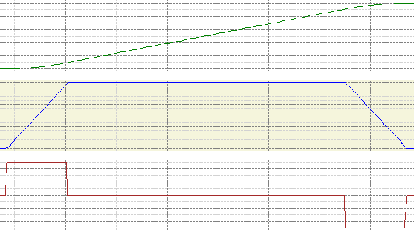 |
Sin² The breaks in the velocity profile are smoothened (by using the sin² function instead of lines) to reduce the jumps in acceleration. The user cannot limit the jerk for this ramp type. The set maximum jerk has an effect only if the acceleration does not equal zero at the beginning of the movement and the interrupted deceleration and acceleration ramp cannot be continued seamlessly. Then, taking the jerk limit into account, the acceleration is decreased to zero before the current movement is started. As compared to the trapezoidal velocity profile, the deceleration takes more time in this case. | 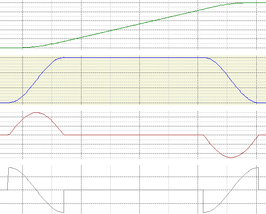 |
Quadratic The acceleration is partially linear and continuous and the jerk has jumps. The velocity consists of quadratic and linear segments. | 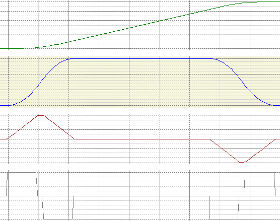 |
Quadratic (smooth) The linear acceleration ramps of the quadratic ramp type are replaced by a "smooth" function with a slope value is zero at the beginning and end. As a result, the jerk is also continuous. Note: If a movement is interrupted, then jumps in the jerk can result. | 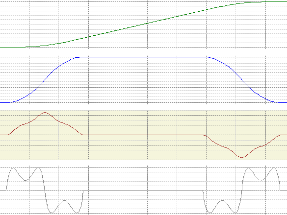 |
For more information, see the following: Interruption of Movements