Tab: Online

General information about the recording

Header

Project path – Creation date and time (example: D:\\proj\\test1.project - 12/26/2014 09:28:14)

Device

Target device where the application is running (example: Device (XY Zxxx V2.1))

Application

Application for the measurement results (example: Device.Application_xy)

Compiler version

Compiler version for the project (example: 3.5.6.0)

Task

Task selected in the settings (example: MainTask)

For instrumentation only:

Number of instrumented POUs

Number of POUs selected in the Profiler settings in POU selection

Example: 5

Cycle

Number of the current cycle, incremented at the start of recording

Example: 2431

Duration

Duration of all calls of the current recorded cycle

Example: 266.318 µs

Time

Time format for the display of the results; internally calculated assignment to the system ticks; defined in the Profiler settings in Snapshot appearance

Example: 1 ms = 3385266 ticks.

Start time of the measured cycle

Start time of the measurement

Example: T#1h50m31s25ms

Current time on device

Time of day

Example: T#4h10m38s47ms - 02/08/2019 11:13:50

Recording mode

Recording mode; defined in the Profiler settings in Instrumentation parameters

Example: Record next cycle

Buffer size

Buffer size for the number of recorded runtimes per cycle; defined in the Profiler settings in Instrumentation parameters

Example: 10000.

For sampling only:

Task cycle time

Interval set for the task to be sampled in its configuration (example: 20 ms)

Number of cycles

Total number of cycles where samples were taken

Example: 3924

Number of sampled POUs

Number of POUs called by the task to be sampled

Example: 11

Total number of samples

Total number of samples (determined call trees)

Example: 2889

Number of busy samples

Number of samples that the POU was currently busy with

Example: 108

Number of idle samples

Number of samples that the POU was currently busy with (IDLE)

Example: 6533

Number of faulty samples

Number of samples that failed (failed)

Example: 4

Number of missing samples

Number of samples that could not be transferred to the development system

Example: 0

Busy cycle time

Time span during the cycle in which the task is running (average value)

Example: 283.000 µs

Idle cycle time

Time span during the cycle in which the task is not running (IDLE) (average value)

Example: 19.716 ms

Recording condition

Condition (Boolean expression) for starting the recording; defined in the Profiler settings in Recording

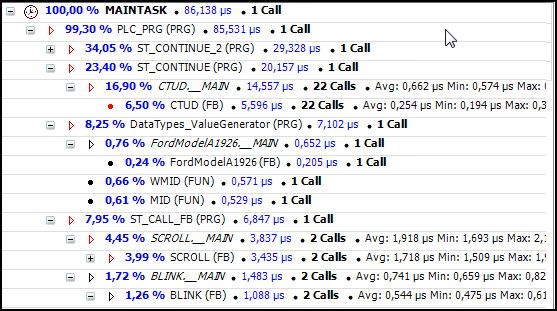
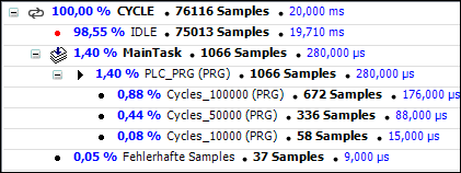
This hierarchical tree structure shows all calls that have been made to the selected task during the measurement period.

Calls in libraries are not displayed.

The top entry shows the name of the task. In the second line, the percentage of samples in which the POU was not busy is shown for the method of sampling with IDLE.

Each node in the call chain displayed below it corresponds to a specific POU call and provides the following information about the current and previous measured times and number of calls:

For both instrumentation and sampling methods:

For the instrumentation method only:

For the sampling method only:

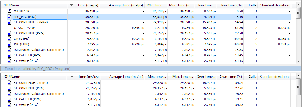
All instrumented POUs are listed. For each POU, you see the number of Samples and the Time (ms/µs) of all recorded calls.

The Functions called by <POU name> list in the lower part of the view always shows the POU calls of the POU currently selected in the list above. Double-clicking a line in the lower list selects the corresponding entry in the upper list.

POU Name

Name and type of POU (example: PLC_PRG (PRG))

Time (ms/µs)

Total time elapsed in the call (example: 85.531 µs)

Average time

Min. time (ms/µs)

Max. time

Average, minimum, and maximum execution time of this call in "ms" or "µs" (example: Avg: 0.254 µs, Min: 0.194 µs Max: 0.3µs)

Own Time (ms/µs)

Own Time (%)

Time that the POU call has spent, excluding the time spent by all POU calls from this POU.

Percentage of the own time to the total time

Calls

Number of calls of this POU in this cycle in this call tree (example: 22 Calls)

Standard deviation

Standard deviation of the average execution time (example: 0.128 µs)

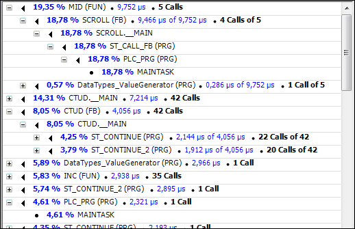
This is a reverse view of the call tree. This means that you can trace all calls from a POU call to the beginning of the call chain. The information shown depends on the profiling method.

For both instrumentation and sampling methods:

For the instrumentation method only:

For the sampling method only:

Refresh snapshot

The current measurements are done and displayed. The display is not refreshed automatically.

Save Snapshot

The Save Snapshot dialog opens for typing in a name and description for the snapshot. After you click OK, the current measurement results are saved and can be called again in the Snapshots tab.

Reset

For the sampling method only:

The current measurement is reset and can be restarted.

Start

Pause

For the sampling method only:

Button for starting, pausing, and stopping, the measurement process

Sampling interval

For the sampling method only:

Time period between measurements. The value of the interval set here is synchronized with the entry in the Profiler settings in Sampling parameters.

A random value is generated in the range between 0 and the specified time span. After this time, the task to be measured is paused and recorded. The remaining time until the specified time span elapses until the next random value is generated. This means that it is measured within the time span, but not before the full time span has been reached.

At a sampling interval of 1 ms, 100 measurements should be performed in 100 ms.

Name

The names of the POUs selected for the measurement are shown in the tree structure. The parent objects act as nodes (for example, the name of the application to which they belong).

Number of statements

Total number of statements contained in the POU.

Statements not executed

Number of statements contained in the POU but not executed.

Coverage (%)

Percentage of statements in the POU that are executed. Example: 75 for 75%.

Open POU

The POU selected in the view is opened in its editor. Statements that have been processed are displayed in green. Statements that have not been processed are displayed in red. The POU editor also opens when you double-click a row in the table.

Reset

The measurement results are reset to 0 and the measurement is repeated in the next cycle.

Save Snapshot

The Save Snapshot dialog opens for typing in a name and description for the snapshot. After you click OK, the current measurement results are saved and can be called again in the Snapshots tab.